---

Excel Data Analysis - Sorting

---

---

---

Excel Data Analysis - Sorting

Sorting data is an integral part of Data Analysis. You can arrange a list of names in alphabetical order, compile a list of sales figures from highest to lowest, or order rows by colors or icons. Sorting data helps you quickly visualize and understand your data better, organize and find the data that you want, and ultimately make more effective decisions.

You can sort by columns or by rows. Most of the sorts that you use will be column sorts.

You can sort data in one or more columns by

• text (A to Z or Z to A)
• numbers (smallest to largest or largest to smallest)
• dates and times (oldest to newest and newest to oldest)
• a custom list (E.g. Large, Medium, and Small)
• format, including cell color, font color, or icon set

Sort criteria for a table are saved with the workbook such that you can reapply the sort to that table every time you open the workbook. Sort criteria are not saved for a range of cells. For multicolumn sorts or for sorts that take a long time to create, you can convert the range to a table. Then, you can reapply the sort when you open a workbook.

In all the examples in the following sections, you will find tables only, since it is more meaningful to sort a table.

Sort by Text

You can sort a table using a column containing text.

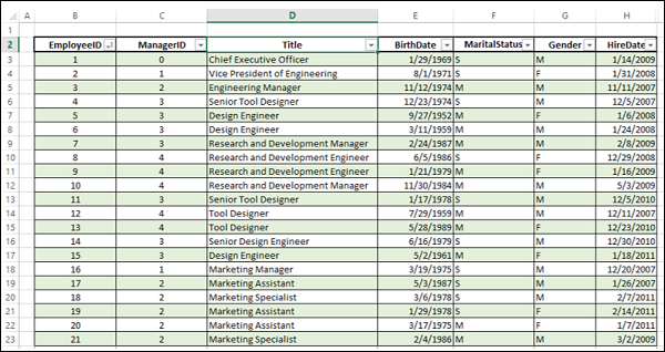
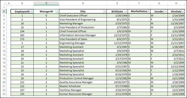
The following table has information about employees in an organization (You are able to see only the first few rows in the data).

• To sort the table by the column title that contains text, click the header of the column – Title.

• Click the Data tab.

• In the Sort & Filter group, click Sort A to Z

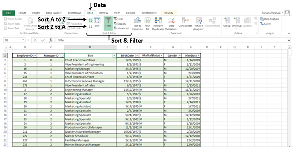
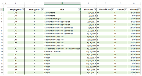
The table will be sorted by the column – Title in the ascending alphanumeric order.

Note − You can sort in the descending alphanumeric order, by clicking Sort Z to A. You can also sort with case-sensitive option. Go through the Sort by a Custom List section given below.

Sort by Numbers

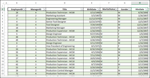
To sort the table by the column ManagerID that contains numbers, follow the steps given below −

• Click the header of the column – ManagerID.

• Click the Data tab.

• In the Sort & Filter group, click Sort A to Z

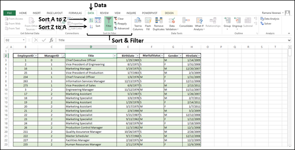
The column, ManagerID will be sorted in the ascending numeric order. You can sort in the descending numeric order, by clicking Sort Z to A.

Sort by Dates or Times

To sort the Table by the column HireDate that contains Dates, follow the steps given below −

• Click the Header of the column – HireDate.

• Click Data tab.

• In the Sort & Filter group, click Sort A to Z as shown in the screen shot given below −

The column – HireDate will be sorted with the dates sorted from oldest to newest. You can sort the dates from newest to oldest, by clicking Sort Z to A.

Sort by Cell Color

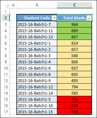
To sort the table by the column total marks that contains cells with colors (Conditionally Formatted) −

• Click the Header of the column – Total Marks.

• Click Data tab.

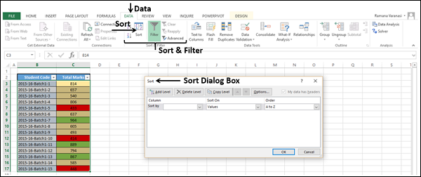
• In the Sort & Filter group, click Sort. The Sort dialog box appears.

• Choose Sort By as Total Marks, Sort on as Cell Color and specify the color green in Order. Click Add Level.

• Choose Sort By as Total Marks, Sort on as Cell Color and specify the color Yellow in Order. Click Add Level.

• Choose Sort By as Total Marks, Sort on as Cell Color and specify the color Red in Order.

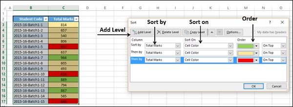
The column – Total Marks will be sorted by the cell color as specified in the Order.

Sort by Font Color

To sort the column Total Marks in the table, that contains cells with font colors (conditionally formatted) −

• Click the header of the column – Total Marks.

• Click Data tab.

• In the Sort & Filter group, click Sort. The Sort dialog box appears.

• Choose Sort By as Total Marks, Sort On as Font Color and specify the color green in Order. Click Add Level.

• Choose Sort By as Total Marks, Sort On as Font Color and specify the color yellow in Order. Click Add Level.

• Choose Sort By as Total Marks, Sort On as Font Color and specify the color red in Order.

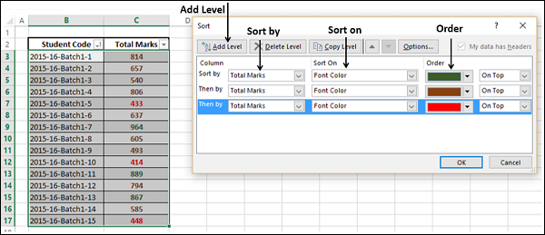
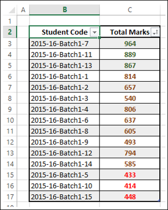
The column – Total Marks is sorted by the font color as specified in the Order.

Sort by Cell Icon

To sort the table by the column Total Marks that contains cells with Cell Icons (Conditionally Formatted), follow the steps given below −

• Click the Header of the column – Total Marks.

• Click Data tab.

• In the Sort & Filter group, click Sort. The Sort dialog box appears.

• Choose Sort By as Total Marks, Sort On as Cell Icon and specify in  Order. Click Add Level.

• Choose Sort By as Total Marks, Sort On as Cell Icon and specify  in Order. Click Add Level.

• Choose Sort By as Total Marks, Sort On as Cell Icon and specify  in Order.

The column – Total Marks will be sorted by Cell Icon as specified in the Order.

Sort by a Custom List

You can create a custom list and sort the table by the custom list.

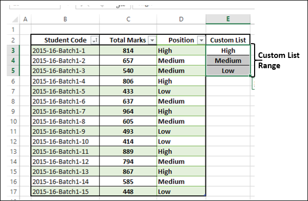
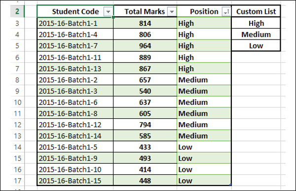
In the table given below, you find an indicator column with title – Position. It has the values high, medium and low based on the position of total marks with respect to the entire range.

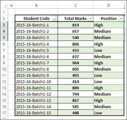
Now, suppose you want to sort the column - Position, with all High values on top, all low values at bottom, and all medium values in between. That means the order you want is low, medium and high. With Sort A to Z, you get the order high, low and medium. On the other hand, with Sort Z to A, you get the order medium, low and high.

You can resolve this is to create a custom list.

• Define the order for the custom list as high, medium and low in a range of cells as shown below.

• Select that Range.

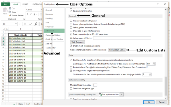
• Click the File tab.

• Click Options. In the Excel Options dialog box, Click Advanced.

• Scroll to the General.

• Click Edit Custom Lists.

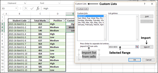
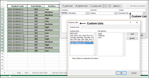
The Edit Custom Lists dialog box appears. The select range in worksheet appears in the Import list from cells Box. Click Import.

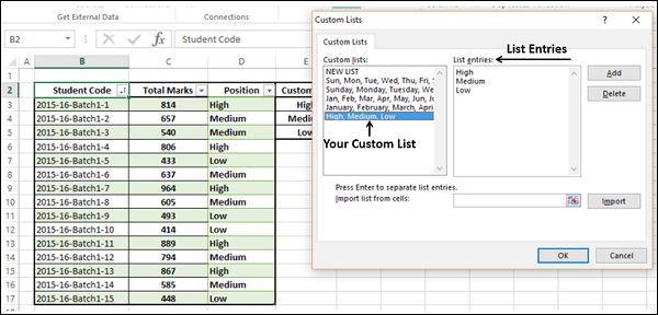
Your custom list is added to the Custom Lists. Click OK.

The next step is to sort the table with this Custom List.

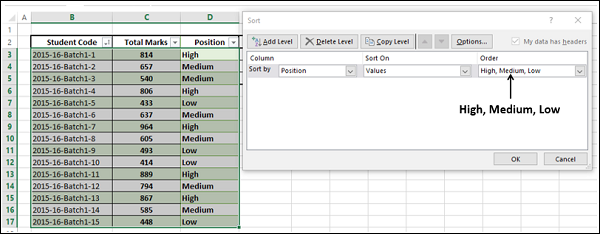
• Click the Column – Position. Click on Sort. In the Sort dialog box, ensure Sort By is Position, Sort On is Values.

• Click on Order. Select Custom List. Custom Lists dialog box appears.

• Click on the High, Medium, Low Custom List. Click on OK.

In the Sort dialog box, in the Order Box, High, Medium, Low appears. Click on OK.

The table will be sorted in the defined order – high, medium, low.

You can create Custom Lists based on the following values −

• Text
• Number
• Date
• Time

You cannot create custom lists based on format, i.e. by cell / font color, or cell icon.

Sort by Rows

You can sort a table by rows also. Follow the steps given below −

• Click the row you want to sort the data.

• Click Sort.

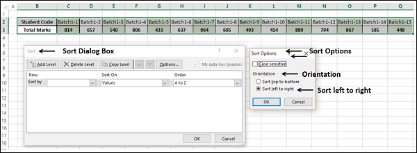
• In the Sort dialog box, Click Options. The Sort Options dialog box opens.

• Under Orientation, click Sort from left to right. Click OK.

• Click Sort by row. Select the row.

• Choose values for Sort On and Largest to Smallest for Order.

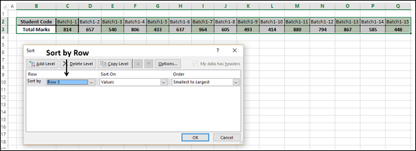
The data will be sorted by the selected row in a descending order.

Sort by more than one Column or Row

You can sort a table by more than one column or row.

• Click the Table.

• Click Sort.

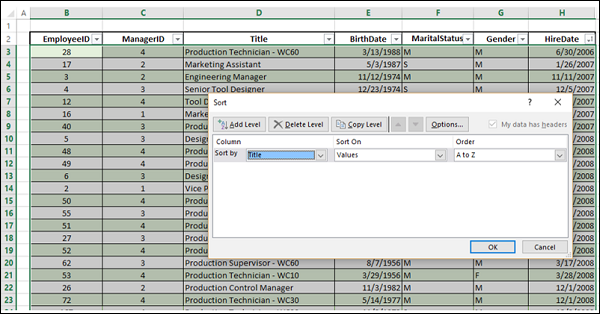
• In the Sort dialog box, specify the column by which you want to sort first.

In the screen shot given below, Sort By Title, Sort On Values, Order A – Z are chosen.

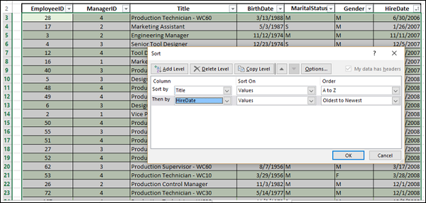
• Click Add Level in the Sort dialog box. The Then By dialog appears.

• Specify the column by which you want to sort next.

• In the screen shot given below, Then By HireDate, Sort On Values, Order Oldest to Newest are chosen.

• Click OK.

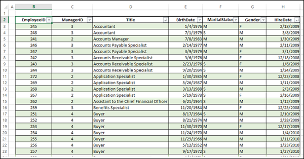
The data will be sorted for Title in the ascending alphanumeric order and then by HireDate. You will see the employee data sorted by title, and in each title category, in the seniority order.

---

---

Frequently Asked Questions

---

---

---

---

---